Sugar menu
  Method of particle size evaluation.
  ICUMSA method GS2-37 leaves the choice of the procedure for mathematical expression of results to the user. The following procedures are described in the appendix:  a) Powers  b) Rens  c) RRSB  d) Butler.  
I would like to discuss a further method of particle size evaluation:

If white sugar passes a sieving station, the particle size distribution will neither follow a Gaussian normal distribution nor a model related with coal comminution (RRSB). Every sugar sample may have its individual cumulative curve. Individual curves can be approximated best by polynoms. With array functions of spreadsheet programs (e.g. MS-Excel or Open-Office/Scalc) it is possible for everybody to evaluate results of analytical sieving by an individual polynomial equation.

For methods based on the Gaussian distribution, results are expressed as M.A. (mean aperture) and C.V. (coefficient of variation = standard deviation, expressed in % of the mean). Other figures of variation, which are not based on the inflexion points of the Gaussian distribution, but derived from an adopted range of variation (rounded to 50±34 %), should be named "C.D. = coefficient of distribution". Thus nobody will be mislead and no Gaussian distribution has to be assumed behind a C.D.

A minimum of six sieves is necessary to use a polynom of the 5th degree. In the ICUMSA example of method GS2-37 seven sieves are used and that is sufficient. In any case the set of sieves must cover 16 % and 84 % of the cumulative % retained, in order to avoid extrapolation. Coarse sieves without retained sugar must be excluded from the regression.

A step-by-step procedure for the ICUMSA example, using MS-Excel or Open-Office/Scalc,  looks as follows:
a) Prepare a table like Table 1a, with powered formulas of column D in columns E to H. The yellow shading indicates the input area. The y‑values in column A represent the sieve aperture size (3 - 9) plus base pan (10) or simply "particle size greater than..." (3 - 10). Column B shows the individual weights for the ICUMSA example. Formulas or constants are written or copied into the white cells of columns C - H.
Table 1a
  A B C D E F G H
1 Aperture size (mm) g retained on sieve cumulative
g retained
cumulative
% retained
       
2 y     x x2 x3 x4 x5
3 0.71 11.3 11.3 11.3 11.3^2 11.3^3 11.3^4 11.3^5
4 0.60 19.3 30.6 30.6 30.6^2 30.6^3 30.6^4 30.6^5
5 0.50 14.6 45.2 45.2 45.2^2 45.2^3 45.2^4 45.2^5
6 0.43 14.6 59.8 59.8 59.8^2 59.8^3 59.8^4 59.8^5
7 0.36 17.6 77.4 77.4 77.4^2 77.4^3 77.4^4 77.4^5
8 0.30 6.3 83.7 83.7 83.7^2 83.7^3 83.7^4 83.7^5
9 0.25 5.9 89.6 89.6 89.6^2 89.6^3 89.6^4 89.6^5
10 0 10.4 100 100 100^2 100^3 100^4 100^5

Table 1b with formulas visible
  A B C D E F G H
1 Aperture size (mm) g retained on sieve cumulative
g retained
cumulative
% retained
       
2 y     x x2 x3 x4 x5
3 0.71 11.3 =B3 =C3/$C$10*100 =D3^2 =D3^3 =D3^4 =D3^5
4 0.60 19.3 =C3+B4 =C4/$C$10*100 =D4^2 =D4^3 =D4^4 =D4^5
5 0.50 14.6 =C4+B5 =C5/$C$10*100 =D5^2 =D5^3 =D5^4 =D5^5
6 0.43 14.6 =C5+B6 =C6/$C$10*100 =D6^2 =D6^3 =D6^4 =D6^5
7 0.36 17.6 =C6+B7 =C7/$C$10*100 =D7^2 =D7^3 =D7^4 =D7^5
8 0.30 6.3 =C7+B8 =C8/$C$10*100 =D8^2 =D8^3 =D8^4 =D8^5
9 0.25 5.9 =C8+B9 =C9/$C$10*100 =D9^2 =D9^3 =D9^4 =D9^5
10 0 10.4 =C9+B10 =100 =D10^2 =D10^3 =D10^4 =D10^5


b) On any free space of the worksheet (e.g. A21:F25) mark an area with 5 rows and 6 columns (Table 2a). Use the mouse with pressed left-button or pressed shift key.
Table 2a
  A B C D E F
... ... ... ... ... ... ...
21  
22
23
24
25


c) After marking, press the F2-key to edit the "input cell" of the marked area (first cell of area in MS-Excel, last cell of area in Open Office) and then type or copy the formula  =LINEST(A3:A10, D3:H10, 1, 1)    to the edited cell of Table 2a, without pressing "Enter". Replace the formula by =RGP(A3:A10; D3:H10; 1; 1)    for German versions.
e) Press "Ctrl" and "Shift" simultaneously and with both keys pressed, additionally press "Enter". This will create an array inside the marked area A21:F25 (Table 2b). Repeat the "three fingers key-press" after any correction (editing) of the marked array via F2-key. The whole array must be deleted in case of a new begin.
  N.B.: It is recommended to use a table corresponding exactly to Table 1 for a first test. Replace the addresses A3:A10 (y-range) and D3:H10 (x-range) for a modified Table 1 logically (base pan included to regression). Menus (Insert, Formula ...) can be used to create the array with some help, but details depend on the program version.
f) The array data are shown in Table 2b, but with some few digits only. The single value in cell A23 is r2. The coefficients a1 - a5 and the constant b will be found at the positions A21-F21.

Table 2b
Pos. of: a5 a4 a3 a2 a1 b
  A B C D E F
... ... ... ... ... ... ...
21 -5,48E-010 +9,29E-08 -4,31E-06 +1.05E-05 -0.0035 0.7532
22 ... ... ... ... ... ...
23 0.999 ... #NV #NV #NV #NV
24 ... ... #NV #NV #NV #NV
25 ... ... #NV #NV #NV #NV


g) The final results are calculated at any free position of the worksheet as follows:
M.A. = F21 + 50*E21 + 502*D21 + 503*C21 + 504*B21 + 505*A21 = 0.47 mm
lim1 = F21 + 16*E21 + 162*D21 + 163*C21 + 164*B21 + 165*A21  
lim2 = F21 + 84*E21 + 842*D21 + 843*C21 + 844*B21 + 845*A21  
C.D. = (lim1 - lim2) / 2 / M.A. * 100 = 40 %

NB: F21, E21... are the cell addresses within Table 2b. With absolute cell addresses ($F$21, $E$21...) the final formulas can be moved within the worksheet and this is more convenient. As long as the same set of sieves is used, new results will be shown immediately after a new input to Table 1, column B.

To exclude coarse sieves from the regression, make use of a) a conditional array which excludes coarse sieves with a cumulative % retained of zero or lower than a selectable value   b) a workbook with different worksheets for different number of sieves   c) editing of the regression formula via F2.

The diagram illustrates the M.A. (50%) and the range of variation (50±34 %) in red, the values for the 7 sieves in blue and the regression curve:

diagram

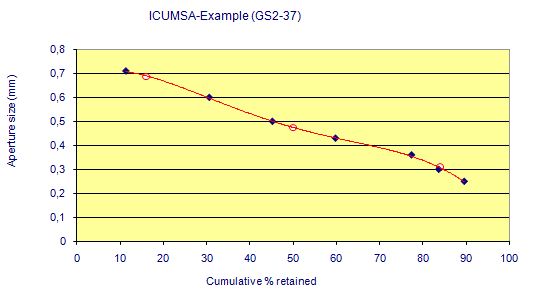
The M.A. result of the Powers method in the ICUMSA example is 0.49 mm, which differs from the polynomial result (0.47 mm). But from figure 1 in the method description of "GS2-37" it is evident that two points near 50 % are outside the straight line.

What would happen with the Powers method, if a sieve will show - by pure chance - a cumulative weight of 50.00 %, which is M.A. per definition ?

Analysts could draw a line away from this important sieve (point) and could state another value of M.A. from the regression line. The same could happen with other linear regression models.

But the polynomial evaluation will indeed show an M.A. close to the sieve which had - by pure chance - 50.00 % of cumulative weight.

According to a discussion with G. Pezzi, the base pan should be included to the polynomial regression.
Original version   2004-08-21  
Update after a discussion with G. Pezzi   2006-04-06
Update after a further Feedback  2010-06-07 G. Pollach